matplotlib Reference Sheet

More Matplotlib

Reference page on most common commands of the matplotlib Python module.

Input

\[\sin x=\sum_{n=0}^{\infty}(-1)^n\frac{x^{2n+1}}{(2n+1)!}\]

import matplotlib.pyplot as plt
from math import*
import numpy as np

# data
r=range(0,370,10)

x=[j for j in r]
y=[j*pi/180 for j in r]
s=[sin(j) for j in y]
c=[cos(j) for j in y]

t1=[tan(j) for j in y if j<90*pi/180]
x1=[j for j in r if j<90]

t2=[tan(j) for j in y if 90*pi/180<j<270*pi/180]
x2=[j for j in r if 90<j<270]

t3=[tan(j) for j in y if j>270*pi/180]
x3=[j for j in r if j>270]

# plotting
plt.plot(x,s,x,c)
plt.plot(x,[s[j]*c[j] for j in range(len(x))],'r',label='$sin x cos x$')
plt.plot(x1,t1,'g')
plt.plot(x2,t2,'g')
plt.plot(x3,t3,'g')


# axis and figure properties
plt.grid()
v=[0,360,-3,3]
plt.axis(v)
plt.title('A Plot of Trignometric Functions\n',fontsize=16)
plt.xlabel('$x$, deg')
plt.ylabel('trg $x$,')

# advanced a little
ax=plt.gca()
ax.legend(('$\sinx$','$\cosx$','$\sinx\cdot\cosx$',r'$\tanx$')) #latex
ax.axhline(y=1,color='k')
ax.axhline(y=-1,color='k')
ax.axvline(x=180,color='pink') #for vertical line

yticks=ax.get_yticks()
yticks=np.append(yticks,[-1,1])
ax.set_yticks(yticks)

xticks=np.array([j for j in range(0,370,45)])
ax.set_xticks(xticks)

ax.text(0.5, 0.9, 'Using\nMatplotlib', horizontalalignment='center',verticalalignment='center', transform=ax.transAxes)
#ax.annotate('$180^o$',[170,0])
plt.plot(180,0,'o',color='red')
plt.show() 

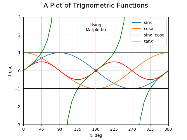
Output

The result is shown below

Appendix

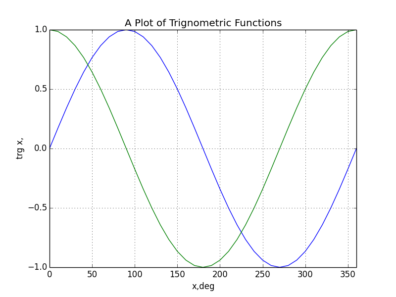
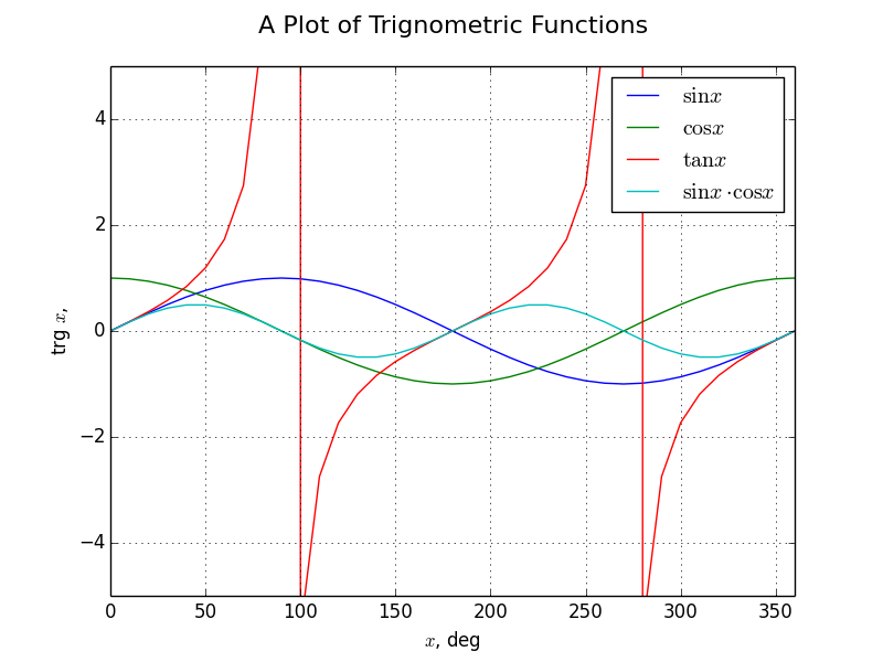
Earlier Versions

See the evolution of this file below

Note to self

You can publish equations like this on HTML from here